Archie's Relationships Clarified

Robert C. Ransom

Table of Retrievable Contents:

Figure 1

A CLARIFYING CONCEPT OF ARCHIE'S RESISTIVITY RELATIONSHIPS AND PARAMETERS.

A MODEL AND DISCUSSION

Within the text, clicking on the bold terms FIGURE (*) and APPENDIX (*) will take you to the specific page of interest. Use your browser's back button to return to your previous page.

Back

Figure 2

Figure 3

Figure 4

Figure 5

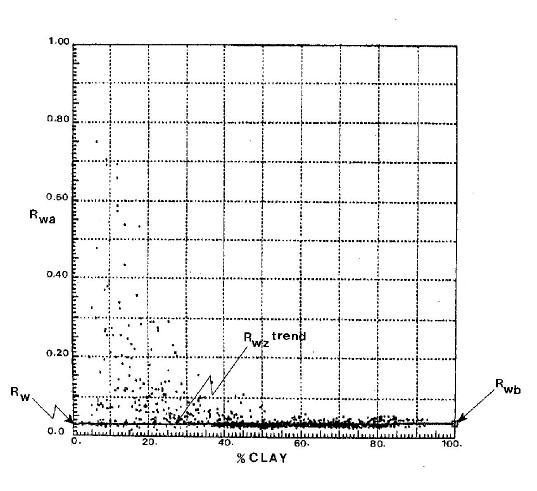
Figure 1. A graphical representation of the model. R_t varies with oil saturation and distribution. Slope CG representing exponent n varies with the electrical interference caused by the presence of oil regardless of saturation value. Swt is estimated by the downward projection of the intersection of the slope CG with resistivity level R_t . See text for full explanation. Based on Ransom (1974,1995). This model can be used with measurements responsive to oil and gas other than resistivity.

Figure 2. When S_wt = 1.0. A detailed portion of the graphical model showing how R_we results from a mixture of waters R_w and R_wb in a shaly sand. The effect of the more conductive pseudo water represented by R_wb produces the typical a multiplier of R_w. This figure and its resulting Rwe corresponds to Eq. (1a) only. Exponent m is an intrinsic property of the rock. Based on Ransom (1974).

Figure 3. An insulating cube with a 20% void filled with water. Electrical-survey current is flowing through the cube from top to bottom. This cube is a visual aid in the development of the formation factor. See text for discussion. From Ransom (1984, 1995).

Figure 4. A crossplot illustrating the iteration of S_wt for the value of S_wt that satisfies both sides of Equation (4b). See the text for discussion.

Figure 5. The crossplot of R_wa versus Clayiness where the identified trend is extrapolated in both directions to evaluate R_w and R_wb at 0% and 100% clayiness, respectively. See text for discussion. From Ransom (1995), courtesy of John Wiley & Sons, Inc.

Back

Figure 6

Figure 1 Reversed Format

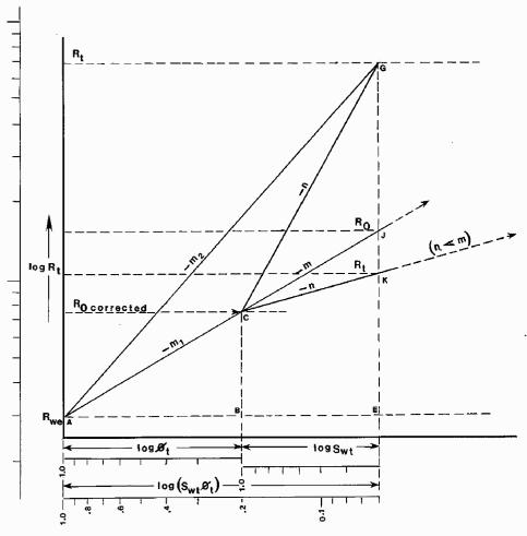
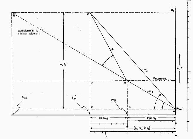
FIGURE 1 reversed format. Same as Figure 1 above, but reversed for convenience of readers familiar with left-facing format.

Figure 6. This figure, similar to Figure 1, shows that when n < m, R_t at K has a lower value than R₀ at J for equivalent water volumes at all values of porosity and saturation. In nature and in the laboratory, this is an impossibility. Any condition for slope n to be less than slope m is contrary to the laws of physics and the fundamentals of resistivity analysis. See APPENDIX (D) for a detailed explanation.

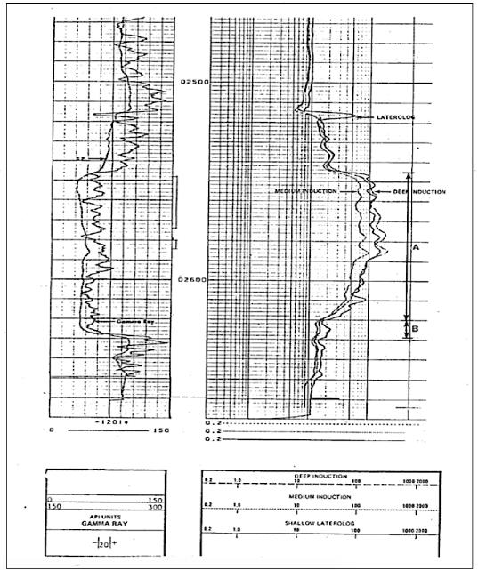
Figure 7. Well 1. The well and reservoir bed in this figure and the following Figure 8 were drilled in the same field. Zone A in this bed was tested over the intervals marked in the depth track and produced much water and little or no oil. No other information is available. Why did Zone A not produce oil? See text for discussion.

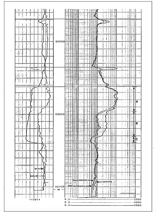
Figure 8. Well 2. The well and reservoir bed in this figure and the preceding Figure 7 were drilled in the same field. No other information is available for this well. Would Zone A produce oil? See text for discussion

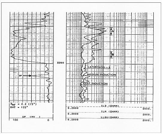
Figure 9. Well 3. An example of a resistivity well log showing the presence of both water and oil in a quality reservoir bed exhibiting considerably lower resistivity than in Wells 1 and 2. Zone A will produce water-free oil. Why? Courtesy of Schlumberger.

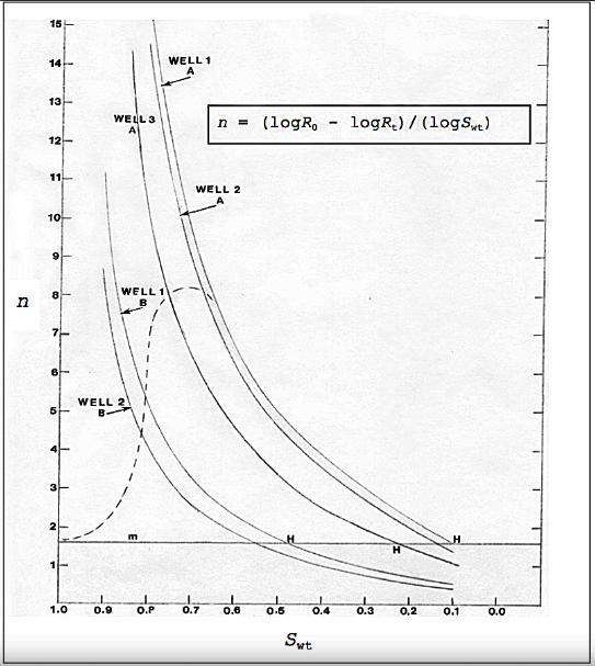
Figure 10. Effectiveness of electrical interference by oil in oil-wet and water-wet rocks. This figure is a chart of the behavior of S_wt in response to the calculated values of exponent n (solid lines) from Well 1 (Figure 7), Well 2 (Figure 8), and Well 3 (Figure 9). This behavior is predicted by slope CG of triangle CDG of the model in Figure 1. See text for discussion and limitations of n.

Figure 7

Figure 8

Figure 9

Figure 10